Derive negative-tail cancellation, underflow, and stable log evaluation from the Gaussian EI integral; reproduce scalar checks and separate batch approximations, noise, budgets, and scientific validation.
An automated experimental system faces two optimization problems: constructing a posterior from observations, and choosing the next experiment from that posterior. The second can require its own nonconvex search. If acquisition values and gradients have already rounded to zero, a better predictive model does not necessarily let the selection program make progress.
This article examines Ament et al.'s Unexpected Improvements to Expected Improvement for Bayesian Optimization, published at NeurIPS 2023. The preprint first appeared on October 31, 2023; the version read here is v3, dated January 7, 2025. This is not a new 2026 release. We focus on analytic single-point LogEI: avoiding numerical degradation of Expected Improvement (EI) without changing the predictive posterior. The derivations and numerical checks address that problem, rather than establishing benefits in physical scientific experiments.
1. Minimal baseline: one experiment from the same posterior
Let continuous experimental conditions be \(x\in\mathcal X\subseteq\mathbb R^d\), and maximize a standardized, dimensionless utility \(f(x)\). Initially restrict the setting to one objective, one point per selection, and noiseless observations. Given data \(\mathcal D\), the latent function at a candidate has a Gaussian posterior:
Here \(\mu\) is its mean and \(\sigma\) the uncertainty standard deviation of the latent function, rather than measurement noise automatically added to a future observation. \(b\) is the best known function value, fixed throughout the current inner selection problem. It does not change with candidate location. \(b,\mu,\sigma\) must share an output scale. If utility has physical units, first choose a fixed reference unit independent of the candidate before taking logarithms; units must not determine the ranking.
Greedy selection of the largest posterior mean can overlook uncertain candidates. EI scores the posterior expectation of the positive improvement over the incumbent. Under these restricted assumptions it measures the expected increase in the best value after the next evaluation; it is neither general information gain nor a probability of scientific discovery. Frazier's Bayesian optimization tutorial supplies background on this baseline and extensions such as noise.
In a continuous domain, the \(\operatorname{argmax}\) generally has no direct analytic solution, requiring initial candidates, restarts, and local optimization. A finite molecular library can instead be scored exhaustively, but numerical zeros can still create many false ties. The failure discussed here occurs at selection, before any new experimental data are collected.
2. Deriving EI and its gradient from a Gaussian integral
Write \(f=\mu+\sigma Z\), with \(Z\sim\mathcal N(0,1)\), and define \(z=(\mu-b)/\sigma\). For now take \(\sigma>0\). \(\phi\) and \(\Phi\) are the standard normal density and cumulative distribution function. Integrating only the region above the threshold gives:
The partial derivatives have a simple interpretation: increasing either the mean or uncertainty while holding the other fixed increases EI. The gradient with respect to experimental conditions also passes through the model:
A small EI value and a truly zero gradient with respect to \(x\) are different conditions. Even when \(\sigma>0\), \(\nabla_x\mu\) and \(\nabla_x\sigma\) can vanish or cancel. LogEI removes neither true stationary points nor the difficulty of global optimization. Numerical stabilization has something to repair when meaningful changes exist but their numerical representation suppresses them.
3. Why is the negative tail difficult to evaluate?
For \(z=-a\), \(a>0\), the candidate mean lies \(a\) posterior standard deviations below the incumbent. Then \(h(-a)=\phi(a)-a\Phi(-a)\): two nearly equal terms are both much larger than their difference. Subtraction loses significant digits, and the exponential scale can additionally fall outside floating-point representation. More restarts do not guarantee recovery of information already lost numerically.
Change variables to the positive excess \(s\), then let \(u=as\) in the same integral:
This expression does not subtract nearly equal numbers. As \(a\to\infty\), expand the second exponential and use \(\int_0^\infty u^k e^{-u}\,du=k!\) to obtain the asymptotic expansion:
The scale \(e^{-a^2/2}/a^2\) is inherent in EI. LogEI does not claim that these candidates have a high probability of improvement. It preserves numerical distinctions and usable derivatives between them. The corresponding logarithmic scale is:
This is a negative-tail asymptotic, not an exact expression for every \(z\). In particular, substituting \(\log|z|\) when \(z\) is near zero is inappropriate. An implementation needs stable expressions for different regions.
4. Reformulate before exponentiating, rather than logging a zero
When \(\sigma>0\), EI is strictly positive and the monotonicity of logarithms gives:
This concerns global maximizing sets under the same posterior and candidate domain. Finite precision, local search, stopping thresholds, and restart strategies can still yield different selected points. Nor does log(max(EI, tiny)) solve the problem: clipping makes a region constant, losing the original ranking and gradient.
The pinned BoTorch analytic implementation uses three regions: direct evaluation for \(z>-1\); a scaled complementary error function and a stable logarithmic difference for more negative inputs; and a leading asymptotic term in the extreme tail. The middle region can be written as:
Here \(\operatorname{erfcx}(v)=e^{v^2}\operatorname{erfc}(v)\) needs a stable special-function implementation, such as SciPy's erfcx. Computing an underflowed erfc before multiplying by the exponential defeats the purpose. log1mexp uses log1p or expm1 to avoid cancellation when \(w\) is near zero. Further into the tail, \(w\) itself approaches zero beyond available resolution, necessitating the third branch. Thresholds depend on dtype.
The following illustrates input/output relationships only; no model fitting or automatic differentiation was executed. For a single-output model, candidate input has shape \((R,1,d)\): \(R\) candidates, one point per group. Removing the two singleton output dimensions gives mean and variance arrays of shape \((R,)\):
posterior = model.posterior(X, observation_noise=False)
mu = posterior.mean.squeeze(-1).squeeze(-1)
sigma = posterior.variance.squeeze(-1).squeeze(-1).sqrt()
z = (mu - b) / sigma
score = log(sigma) + stable_log_h(z)
x_next = multistart_maximize(score, bounds, restarts, budget)
Check that broadcasting the mean, standard deviation, and incumbent does not silently introduce another dimension. Vectorized code must also mask hazardous inputs in inactive branches to avoid contaminating automatic differentiation. Degenerate \(\sigma=0\) points require the limit \(\max(\mu-b,0)\), usually zero at noiseless evaluated points. Artificially increasing all standard deviations is not the numerically equivalent reformulation discussed here.
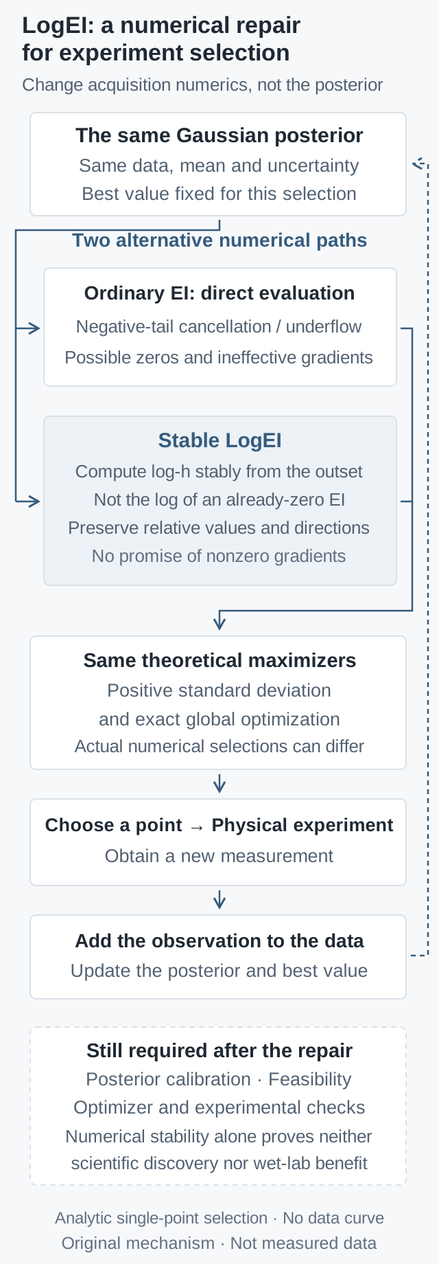
Original mechanism, not an experimental curve: ordinary EI and stable LogEI share the same posterior and fixed incumbent. Stable evaluation avoids numerical degradation from negative-tail cancellation and underflow. Their theoretical maximizing sets agree at positive standard deviation, but practical numerical searches can choose different points. New experimental observations drive posterior updates. Calibration, feasibility and experimental benefit require separate validation.
5. Executed check: direct EI reaches zero while its log remains distinguishable
This section executes independent scalar numerical calculations, not GP training, BoTorch autograd, complete BO, or physical experiments. Fix \(\sigma=1\) and evaluate eight specified \(z\) values. The direct float64 baseline uses \(\Phi(z)=\tfrac12\operatorname{erfc}(-z/\sqrt2)\), avoiding artificial additional CDF cancellation from 1 + erf.
The stable path is an original scalar reference implementation using SciPy special functions and branching. Its approach is checked against the official source, without claiming bit-for-bit reproduction of Torch. High-precision mpmath references evaluate the Gaussian closed form and independently cross-check the positive integral in the negative tail, repeating at increased precision. Dependencies, commands, and all checks are in the downloadable reproduction script.
These results were executed locally rather than transcribed from the paper: CPython 3.12.14, SciPy 1.16.2, mpmath 1.3.0, NumPy 2.3.5, macOS arm64, and a 53-bit binary significand. The main table fixes \(\sigma=1\) and checks \(z\in\{1,0,-1,-5,-10,-20,-40,-100\}\). High-precision references are repeated at target decimal precisions of 80 and 160 digits, each with 40 internal guard digits; the negative-tail positive integral is cross-checked against the closed form. All cases pass the script's thresholds. This checks consistency under precision refinement; it is not a rigorous error certificate from interval arithmetic.
Across the main table, the largest absolute difference between the stable logarithm and the 160-digit reference rounded to float64 is \(1.82\times10^{-12}\). The largest relative difference of the mean partial derivative from its reference, holding \(\sigma,b\) fixed, is \(1.51\times10^{-12}\). Float64 central differences separately check the scalar logarithm with step \(10^{-5}\max(1,|z|)\), giving a maximum relative difference of \(1.30\times10^{-11}\). A zero difference from a rounded reference does not establish exact equality at infinite precision. Additional checks cover the extreme-negative branch, positive affine output scaling, ranking, and explicit rejection of zero standard deviation. The code does not fit a GP, optimize an acquisition, execute autograd, or measure GPU latency.
The derivative shown is \(\partial\log\mathrm{EI}/\partial\mu\), holding \(\sigma,b\) fixed, rather than the full experiment-condition gradient \(\nabla_x\log\mathrm{EI}\). Values are rounded for display; the reproduction script emits full precision and every assertion.
Executed scalar comparison at standard deviation 1; not scientific experimental data.
\(z\)
Direct float64 EI
Stable log EI
\(\partial_\mu\log\mathrm{EI}\)
1
1.083315471
0.0800262188493
0.776638725202
0
0.3989422804
-0.918938533205
1.25331413732
-1
0.08331547059
-2.48512102571
1.90427123333
-5
5.346165534e-08
-16.7443011627
5.36181624129
-10
7.474560255e-25
-55.5531220361
10.1943830334
-20
1.370012495e-90
-206.917838509
20.0992628111
-40
0
-808.298568357
40.0499066576
-100
0
-5010.1295788
100.019994004
The paths evaluate the same mathematical EI, not two different models. A zero in the table means that this direct expression cannot distinguish the value in the stated environment, not that improvement has exactly zero probability. A stable logarithmic value is also no evidence of a new material, improved drug activity, or lower experimental expense. This test validates the numerical representation alone.
Autograd validation would require separate model-level gradient and directional-derivative checks. Freeze the posterior, share initial conditions and restart budgets, and compare candidate rankings against high-precision references. Use appropriately scaled finite differences away from branch boundaries, then inspect the resulting selections. These are proposed follow-up tests. Only the scalar checks above were executed.
6. Batches, noise, and constraints: where exact equivalence ends
The analytic single-point result does not transfer unchanged to a batch of experiments. For \(X=(x_1,\ldots,x_q)\), sample from the joint posterior to preserve candidate correlations. Batch EI is:
A Monte Carlo estimate from \(S\) fixed joint draws includes \(1/S\). If none of a draw's candidates exceeds \(b\), the positive part and maximum create truly zero sample-level gradients; this is more than floating-point underflow. The paper and BoTorch's qLogEI implementation therefore add smoothing. That differs from the exact monotonic transformation for analytic single-point LogEI. Temperatures, tail approximations, sample count, and batch size must be recorded.
Here \(\widetilde U_s(X)>0\) is a smoothed sample improvement utility. The expression describes a stable log sample average, not the entirety of qLogEI. Independent draws for each candidate cannot be passed off as a correct joint batch value. Nor should larger batches conceal a larger physical evaluation budget.
With measurement noise, the best observed outcome may be a lucky draw. Treating it as a certain \(b\) changes the decision problem; consider uncertain latent baselines, replicate measurements, and noisy EI methods while checking output and noise conventions. Constraints likewise go beyond box bounds: enforce known hard limits and model unknown feasibility. A simple product of EI and feasibility probability requires the corresponding conditional-independence assumptions. Taking logs does not automatically satisfy experimental safety, consumables, or shared batch-resource constraints.
7. How should a scientific experimental loop be evaluated?
Account for computational and physical-experiment budgets separately. A standard dense GP with \(n\) observations typically uses \(O(n^3)\) time and \(O(n^2)\) storage for a Cholesky factorization. With that factor available, a single-point variance triangular solve is typically \(O(n^2)\). Stable analytic log-h adds constant-order scalar work without changing these orders; this is not a wall-clock speedup guarantee. Positive-part and maximum operations on batch draws take \(O(Sq)\), excluding joint sampling and model evaluation, and cannot be called the cost of the whole algorithm.
A proposed comparison has three layers. First freeze the posterior and check values, derivatives, rankings, and numerical boundaries. Next use a verifiable offline objective or simulator with shared initial data, true evaluation counts, feasible domains, model-fitting settings, restarts, and inner evaluation budgets; inspect best achieved values and failures. Only then test prospectively in a scientific experimental system with independent outcome acceptance. If models, noise assumptions, or filtering rules also change, their entire benefit cannot be attributed to LogEI.
Check design leakage in scientific evaluation. Training a surrogate on a complete experimental table and searching that same surrogate establishes optimization of that surrogate. Features, kernels, standardization, or screening based on outcomes available only later invalidate a deployable historical replay. Freeze available information by time or independent batch, retaining failures, measurement batches, and replicates. Prospective comparisons should share starting knowledge and randomize allocation or carefully address instrument, batch, and condition differences. Report qualified experiments, consumables, time, and independent retesting alongside outcomes, rather than only best-so-far curves.
The chain to test is whether numerical accuracy improves inner selection; whether better selection under a credible posterior improves decisions; and whether those decisions yield independently reproducible science under matching resources. Each link can fail. The executed test here covers scalar arithmetic in the first layer; the other layers are evaluation proposals.
8. What cannot numerical stabilization repair?
If the posterior confidently misclassifies an out-of-distribution candidate as unpromising, LogEI may optimize that mistaken judgment more faithfully without recovering scientific knowledge. A proxy detached from the real experiment, unmodeled measurement drift, missing feasibility conditions, or a local stationary point remains a problem. Tiny gains may also indicate insufficient remaining task value. The ability to represent small numbers is not a reason to spend experimental budget indefinitely.
Predefine stopping or model-revision conditions: acceptable reference error, whether credible candidates' expected gains justify costs, independent retests supporting the posterior, and fixed-budget outcomes exceeding a shared baseline. A tiny EI at one candidate and absence of worthwhile candidates across the feasible domain are separate judgments.
The AI4S lesson is to establish that the computer actually executes the claimed selection policy before judging its intelligence. A stable acquisition function supplies a reliable part of decision implementation. New experimental observations, credible uncertainty, and reproducible outcomes make that implementation a scientific loop.
Citation metadata were checked with citation-management tooling; its software attribution is Scientific Agent Skills. This tooling citation is not evidence for LogEI's mechanism or experimental benefit.