报告的 AVI 拆分与测试按位点去除训练/验证重叠,即使 ALT 不同也排除,indel 还扩展到覆盖区间;验证使用功能与关联数据来选模。这个防泄漏措施值得保留,但不能据此声称底层 AlphaGenome 从未见过该基因组区域:轨道预测的折间留出与用于变异评分的蒸馏模型是不同设置。建议新增基因座、时间和实验来源对照,辨认上下文记忆、任务迁移与真实增量。报告第 21–22、28 页;底层模型的训练与蒸馏。
Follow AlphaGenome Atlas from paired tracks and 18 features through frequency proxy labels, raw logits and PHRED ranks, testing the boundaries of probability, attribution, coordinates and compute budgets.
What should AVI 20 mean for a noncoding variant? A tempting leap is to read a high whole-genome rank as a 99% probability of causing disease. AlphaGenome Atlas connects molecular predictions, candidate ranking, and mechanism exploration. That connection depends on preserving what each score actually measures. We start from a minimal REF/ALT comparison, follow 18 features into a raw logit and then a PHRED rank, and provide executable mathematical counterexamples.
The Atlas resource was released on September 8, 2026; the associated medRxiv v1 was posted on September 20 and remains a preprint. The version examined here is the report linked by the official announcement, particularly Methods on pages 18–28. The foundational AlphaGenome paper appeared in Nature on January 28. This is an interpretation of existing public work rather than an announcement of a new event today. Resource release; Official report; Preprint; Foundational paper.
1. Minimal baseline: two predictions in matched context
AlphaGenome accepts approximately 1 Mb of DNA context and predicts molecular-assay tracks, including RNA expression, chromatin accessibility, and splicing. It predicts patterns of assay readouts rather than directly consuming an individual’s full genetic and clinical context to return a disease posterior. Output heads have different resolutions; not every modality is a base-resolution, one-dimensional expression signal. Model and output heads.
For a variant \(\nu\), prepare reference and alternative sequences in the same context, holding other conditions fixed. Modality \(m\) yields \(Y_m^{\mathrm{ref}}\) and \(Y_m^{\mathrm{alt}}\). A specified scorer, spatial mask, aggregation, and transformation produce \(z_{m,c,g}\). Tissue or track \(c\) and gene or position \(g\) are modality-dependent indices. Saying ALT minus REF alone leaves unanswered the order of aggregation and transformation, the gene being compared, and the assay context. Official scoring documentation.
Validate coordinates and metadata first. Atlas precomputation uses GRCh38, which determines REF; N/n bases were not scored, and all substitutions between two nonreference alleles at a position were not computed. Swapping REF and ALT can cause a lookup miss rather than return a value that can simply be negated. The general online prediction interface accepts user-specified REF/ALT, so it cannot be assumed to validate reference-genome consistency for you. Record assembly, alleles, position, scorer, tissue, and annotation version, and actively check REF. In the SDK, Variant position is 1-based and Interval start is 0-based. Report pages 18–20; Pinned FAQ.
2. Eighteen features: what gets compressed?
AVI does not send every tissue track into an unlimited-dimensional classifier. It uses ten AlphaGenome molecular features, four coding-related features, two conservation features, and two indel-type indicators. Coding features include AlphaMissense and three loss-of-function consequence annotations (protein termination, stop lost, and start lost); conservation derives from multispecies alignments. Nine molecular scorers take the maximum absolute effect over relevant tracks, genes, and other dimensions; splicing uses a separate merged feature. With simplified indices:
Only the junction term is divided by five, not the entire splicing sum. Active allele scores describe absolute allelic activity and are excluded from these AVI molecular features. Features are not expressed in one common physical unit; retain each scorer’s meaning. Report pages 22–23.
Maxima solve the engineering problem of compressing many predictions into a small feature vector, while imposing an interpretation boundary. The largest accessibility effect could come from tissue A, and the largest RNA effect from tissue B. Ten maxima are not ten jointly measured effects in one cell state. Absolute values also remove some directional information. To investigate a mechanism, return to the paired predictions for the specific tissue, track, and gene, and check direction and extent.
The ten AlphaGenome molecular features and Cactus conservation use MaxAbsScaler fitted only on training-set maxima:
Here \(\mathcal T\) is the training set, and the denominator is assumed positive. Other features retain their stated scales; do not restandardize all eighteen arbitrarily. Fixed training statistics allow new values outside the training range, so scaling is not itself out-of-distribution calibration. A reimplementation encountering a constant-zero feature needs an explicit policy rather than an inferred official behavior.
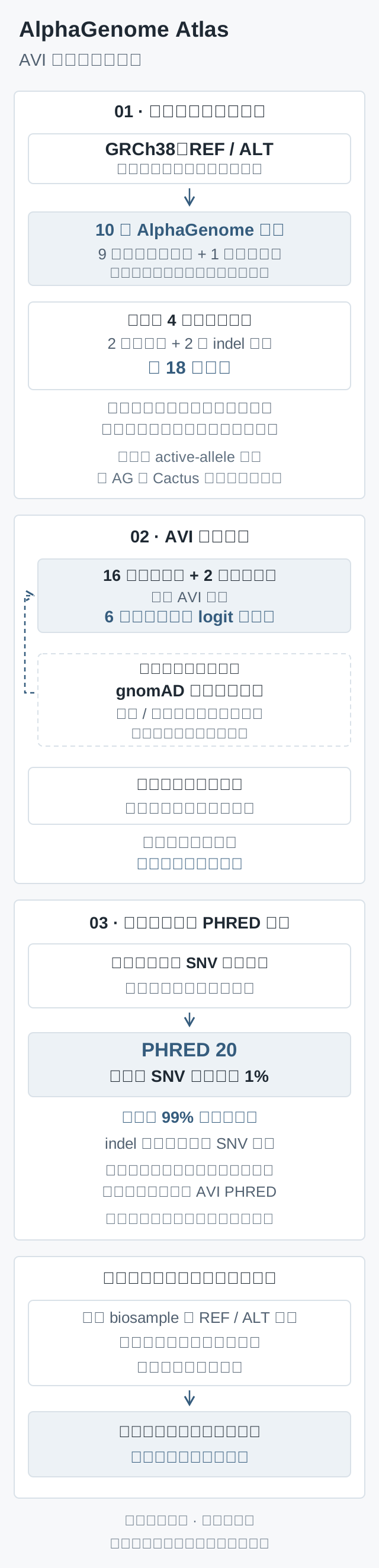
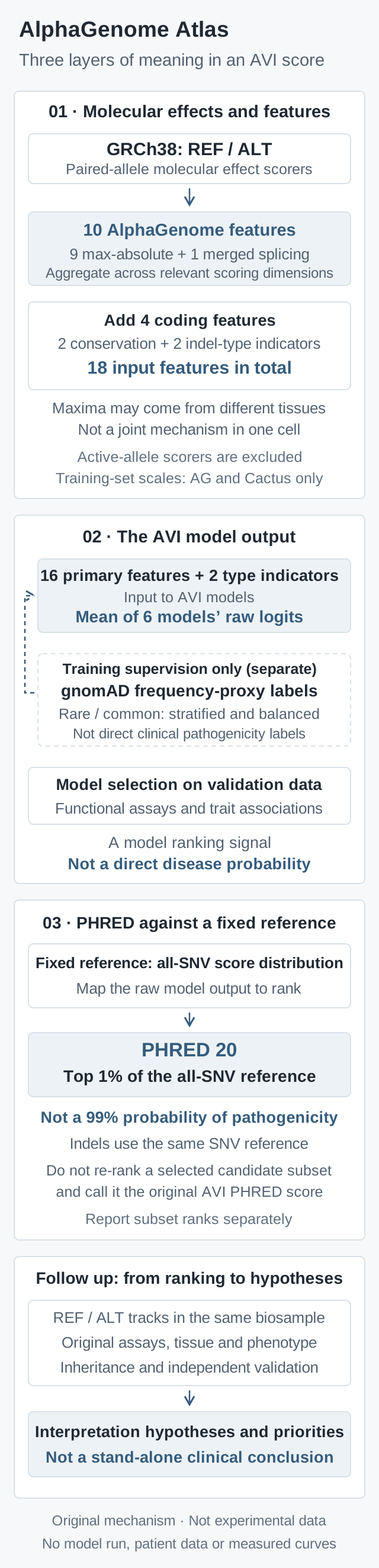
Original mechanism illustration, not experimental data or model-run results. Molecular-effect features, AVI output learned with frequency-proxy supervision, and PHRED rank against the fixed all-SNV reference are different layers. PHRED 20 denotes the reference’s top 1%, not 99% pathogenicity. Cross-tissue maxima do not establish a joint mechanism in one cell, and indels still use the SNV reference. Interpretation and prioritization require paired tracks, original assays and independent contextual evidence; the figure gives no clinical conclusion.
AVI is trained on observed variants in gnomAD v4.1 genome data, with proxy labels derived from FAF95_GRPMAX, the 95% lower bound of the maximum filtering allele frequency across genetic ancestry groups. Variants below 0.001 are proxy impactful; those at least 0.001 and below 0.999 are proxy neutral. This exploits information related to negative selection without establishing that each rare variant causes disease or removing rare neutral variants from the positive class. Report pages 20–21.
SNVs are balanced within 96 reverse-complement-collapsed trinucleotide substitution contexts to reduce local mutational-background confounding. Training indels are balanced by length, restricted to at most 10 bp. Ten resampled sets are used. This reduces some context and baseline-mutation-rate effects, while altering the class proportion and input distribution seen by the model. Balance is a data-construction rule, not a measurement of population disease prevalence.
For proxy label \(y\), training uses binary cross-entropy on the logit:
Even perfectly calibrated \(\sigma(f)\) would answer the proxy-class question under the sampled distribution. To isolate the role of priors, consider a strictly limited hypothetical setting: the label definition and class-conditional distributions remain unchanged, and only the prior shifts from \(\pi_{\mathrm{sample}}\) to \(\pi_{\mathrm{target}}\). Bayes’ rule gives:
This is a general probability derivation here, not an Atlas calibration procedure. With sampling prior 0.5, sampled posterior 0.9, and target prior 0.01, the same-label target posterior is only about 8.33%. Actual Atlas additionally uses context-stratified sampling; more fundamentally, a disease event and a frequency-derived proxy class are different labels. Changing one prior cannot perform either additional conversion.
Nor should the whole study be described as using no functional or clinical data. Gradient training uses frequency proxy labels, but model selection uses independent functional and association validation benchmarks; formal testing also includes ClinVar. Training supervision, validation selection, and test evidence must be recorded separately.
4. Raw logits: conditional weights are not fixed evidence weights
The report denotes primary features by \(x\in\mathbb R^{16}\) and insertion/deletion indicators by \(v\in\{0,1\}^2\). The type vector is zero for SNVs. A conditional hypernetwork, an ordinary linear branch, and an indel offset are combined:
The hypernetwork uses current \(x,v\) to generate nonnegative weights \(w_\phi(h)\) and a bias, so different variants can combine features differently. The ordinary linear branch has no corresponding nonnegative-weight constraint. Six ensemble members average raw logits:
Applying sigmoid to the average logit generally differs from averaging per-member sigmoids; retain the reported order. Pages 24–26 specify architecture and training. The public SDK’s ability to query scores should not be read as release of all AVI training weights.
Another tempting inference is that nonnegative hypernetwork weights force every feature increase to raise the final score. Holding \(v\) fixed and differentiating with respect to primary features gives:
Only the first term is directly constrained by nonnegative weights. Input-dependent derivatives of weights and bias, and the ordinary linear branch, must also be counted. A minimal mathematical counterexample is:
Weight \(e^{-x}\) is always positive, yet the derivative is negative for \(x>1\). This does not reproduce AVI’s learned function; it establishes that positive weights alone are insufficient to prove whole-model monotonicity. An interpretable conditional combination is not a fixed set of additive biological evidence weights.
5. PHRED 20: a logarithmic upper-tail rank
The report converts the mean raw score to PHRED using the distribution of all SNVs: 10 means the top 10%, and 20 the top 1%. Indel raw scores map to the same SNV quantile curve, not to a separate ranking within indels. Figure 1 and pages 3–4.
For explanation, define a finite reference set \(\mathcal R\) of size \(N\), counting every tied score in the upper tail:
Including equality is a teaching convention. The report does not fully disclose backend discrete ties, interpolation, and endpoint handling for AVI, and the code here does not claim a bitwise reproduction. A score inside the reference has a nonzero tail; the teaching code rejects values above its reference maximum instead of silently extrapolating a finite score. A tail fraction of 0.01 gives \(Q=20\). That fraction counts background scores at least as high; no disease label enters the expression.
Consider a purely synthetic reference of one thousand integers, 0 through 999. Ten are at least 990, yielding 20. If only 990 through 999 remain as a candidate set, the same 990 from the same model has upper-tail fraction one and teaching score zero. Reranking a subset changes the reference question and cannot be called the original whole-genome AVI PHRED. In contrast, applying a strictly increasing transformation to both scores and a fixed reference preserves tail ranks. Ranking retains order while discarding the original scale.
Quantity or stage
Reference distribution
Meaning to preserve
Single-scorer quantile_score
Official FAQ: common variants with MAF > 0.01 in any gnomAD v3 population
Relative unusualness for a scorer/track; cannot substitute for AVI PHRED
AVI training proxy labels
gnomAD v4.1 FAF95_GRPMAX threshold and stratified balanced sampling
Proxy target and sampled distribution
AVI PHRED
Ranking of raw scores for all SNVs; indels map to the same SNV curve
Upper-tail position against a fixed background
Disease-event posterior
Real labels, class proportion, and conditional evidence for a specified task
Requires separate validation; cannot be read directly from any preceding rank
Single-scorer quantiles and AVI PHRED are distinct transformations. Both may appear as calibrated scores in interfaces without sharing a reference population. In a candidate list already filtered by frequency, region, or family information, the background changes. The top 1% of all SNVs does not automatically mean a 1% false-positive rate within that list. Pinned FAQ: raw and quantile definitions.
6. What else is needed for a disease posterior?
Let disease-related truth be \(D\), the high-score event \(B\), and the truth proportion in a specified task \(\pi=\Pr(D=1)\). If its sensitivity \(\alpha\) and false-positive rate \(\beta\) are actually known, conditional probability gives:
This follows by decomposing positive hits and negative false alarms. The whole-SNV tail fraction in PHRED is not \(\beta\), and the reported rank does not directly supply \(\pi\) for an individual or task. A second explicitly hypothetical counterexample fixes sensitivity at 0.9 and false-positive rate at 0.01. At truth proportion 0.001 the posterior is approximately 8.26%; at proportion 0.1 it is about 90.91%. These numbers are not AVI experimental or clinical performance; they illustrate how identical conditional rates yield different posteriors in different backgrounds.
A high score can prioritize the next check. Mechanism interpretation still needs tissue, expression and splicing context, the scope of the variant, and independent genetic and experimental evidence. Atlas lists missing cell types, incomplete coverage of some RNA measurements, and no direct modeling of trans regulation among its limitations. A selected case or an AUPRC value does not provide probability calibration for every candidate, ancestry, or application. Report pages 18 and 27–30.
7. Attribution: preserve the raw-scale baseline
Atlas uses expected gradients to approximate SHAP attribution on the raw-logit scale. Methods specify a zero-vector background, but zero input does not imply zero output. To distinguish the complete input from the sixteen primary features, write \(z=(x,v)\) and model output \(F(z)\). Under differentiability, integrability, and exact path integration, a zero-baseline path satisfies (the partial derivative is with respect to the model’s ith input coordinate, evaluated at the path point):
Summation follows from the chain rule and the fundamental theorem of calculus. Actual expected-gradient estimates introduce numerical approximation, so check \(F(0)+\sum_i\phi_i\approx F(z)\) rather than silently removing the baseline. Results and figure captions summarize contributions as summing to the raw score; the derivation here follows the Methods baseline definition without assuming the released model has zero output at zero. Report page 26.
Even approximately additive raw-scale attributions cannot directly become additive PHRED shares after whole-genome ranking and logarithmic transformation, much less shares of disease probability assigned to molecular mechanisms. A conservation-driven high score may offer little specific molecular interpretation. Attribution identifies signals used by the model; causal testing needs different evidence.
8. Compute budget: where does precomputation move the work?
Atlas precomputation avoids rerunning a long-sequence model for each lookup. The report tiles the reference in 128 bp windows, enumerates three ALT bases per non-N position, and caches one REF prediction in a shared approximately 1 Mb context. For \(n\) scorable positions in a window, idealized forward-pass counts are:
A full window has at most 384 ALT sequences: independent pairs require 768 passes and caching gives 385. This is a call-count ledger, not measured approximately twofold acceleration. Prediction heads, memory traffic, batching, compression, and writing outputs still cost time. Some gene-annotation masks are reusable; center and contact-map masks remain variant-specific. Indels are handled separately without this REF caching, and their activation shift/stitch strategy requires three passes. SNV budgets and coordinate rules cannot simply be copied to indels. Report pages 19–20.
Lookup also has a budget. The pinned SDK splits intervals into small chunks, makes paginated concurrent requests, and materializes results. Scorer, tissue, and gene filters affect transferred data and host parsing memory. Querying precomputed values, running fresh online inference, and training AVI locally are different workloads. No such models, services, or whole-Atlas downloads were run or timed here, so no unmeasured end-to-end latency is asserted. Pinned Atlas client.
The teaching tail code sorts its reference once in \(O(N\log N)\) time using \(O(N)\) storage and locates each tail by binary search in \(O(\log N)\). This illustrates separating reference preparation from lookup, not a claim that production Atlas uses this small data structure.
9. Acceptance through testable controls
The accompanying original Python check script uses only the standard library. Run python3 alphagenome-avi-ranking.py. The author actually passed 80 arithmetic checks: reference scores and ties, invariance to increasing transforms, changes under subsetting, logit versus sigmoid averaging, same-label prior correction, hypothetical Bayes rates, positive conditional-weight nonmonotonicity, attribution with a nonzero output baseline, and SNV pass counts. Extreme priors use log-odds to avoid direct-odds overflow. These are synthetic mathematical checks, with no AlphaGenome, AVI, real genomic-variant, or clinical experiment.
A research-use evaluation can prespecify three controls. First, compare frequency and conservation baselines, molecular scorers, and AVI on the same versioned variant cohort, keeping assembly, scorable set, filtering, and sign conventions matched. Report uncovered variants separately rather than assigning zero effect. Second, track which predicted changes are supported by independent tissue or functional experiments, retaining counterexamples and unmeasured outputs instead of selecting one mechanism story. Third, assess ranking and probability calibration separately for a defined target and population, documenting labels, prevalence, and selection. Without the corresponding truth, preserve uncertainty.
AVI splitting and testing remove training/validation overlap by position even when ALT differs, expanding the interval for indels; validation uses functional and association data for selection. Retain this leakage control, while avoiding the claim that underlying AlphaGenome never saw the genomic region. Fold-held-out track prediction and the distilled model used for variant scoring are different settings. Additional locus, time, and experimental-source controls can distinguish context memory, task transfer, and incremental benefit. Report pages 21–22 and 28; Underlying training and distillation.
Acceptance comes down to concrete interfaces. Is a score reproducible with correct coordinates and fixed background? Which tissue, track, and feature drives it? Does independent evidence support those signals? Does ranking improve prioritization within the target candidates, and is probability separately calibrated to the same real target? Answering those questions turns a large precomputed resource into an auditable research priority rather than an overinterpreted scalar.
Citation metadata was checked using the citation-management workflow from Scientific Agent Skills. Its current paper version is v2, revised September 2, 2026. That tool reference documents the research process and is not evidence for genomic or disease conclusions. Kassis et al., Scientific Agent Skills.